Tracking in Computer Vision is the task of estimating an object’s trajectory throughout an image sequence. To track an individual object, we need to identify the object from one image to another and recognize it among distractors.
There are a number of techniques we can use to remove distractors, such as background subtraction, but we’re primarily interested here in the tracking technique known as tracking by detection. In this paradigm, we first try to detect the object in the image, and then we try to associate the objects we detect in subsequent frames. Distinguishing the target object from distractor objects is then part of an association problem — and this can get complicated! You can think of it like “connecting the dots” — which is exponentially more challenging when there are many dots representing many different objects in the same scene. For example, if we want to track a specific car in a parking lot, it’s not enough just to have a really good car detector; we need to be able to tell apart the car of interest from all the other cars in the image. To do so, we might compute some appearance features that allow us to identify the same car from image to image. Alternatively, we can try to track all the other cars, too — turning the problem into a Multi-Object Tracking task. This approach enables more accurate tracking by detection with weaker appearance models, and it allows us to track every object of a category without choosing a single target a priori.
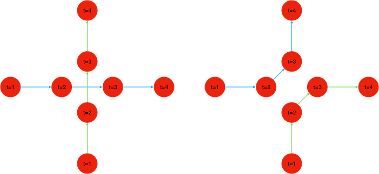
In these figures, we’re trying to track two red dots, simultaneously detected over 4 consecutive frames (t=1,2,3,4). But with only the position and time of detection as information, there are two different sets of trajectories that are acceptable solutions. The two dots may cross paths while maintaining a straight motion like in the left image, or they may avoid each other turning in opposite directions, like in the image on the right. If we were only interested in tracking one of the two dots, the second one would act as a distractor potentially causing a tracking error.
What are the current approaches?
As a still largely unsolved and active area of research, there’s an extensive literature covering different approaches to multi-object tracking. Since 2014, there has even been a standard benchmark in the field, called the Multiple Object Tracking (MOT) Challenge, which maintains datasets that researchers and individuals can use to benchmark their algorithms. We’ll discuss a few common approaches here and present them in a simplified way, but this is far from an exhaustive list. For more, we suggest the following survey from 2017 by Leal-Taixé Laura et al..
Kalman Filtering and Hungarian algorithm
One of the simplest approaches is to try matching detections between adjacent frames, which can be formulated as an assignment problem. In its simplest form, for each object detected at time t, a matching distance is computed with each object detected at time t+1. The matching distance can be a simple intersection-over-union between bounding boxes, or it could include an appearance model to be more robust. An optimization algorithm called the Hungarian algorithm is then used to find the assignment solution that minimizes the sum of all the matching distances. In addition, since most of the objects we are trying to track are moving, rather than comparing the new detection’s position to the tracks most recent known locations, it works better to use the track position history to predict where the object was going. In order to integrate the different uncertainties from this kinematic model and the noise from the detector, a filtering framework is often used, such as a Kalman Filter or Particle Filter.
A more complex but straightforward extension to this approach is to search for an optimal solution over a higher number of frames. One possible way is to use a hierarchical model. For example, we can compute small tracklets between adjacent frames over short, non-overlapping segments, and then try to match tracklets between consecutive segments. The Hungarian algorithm can be used again if we can come up with a good distance-matching function between tracklets.
Multi Hypothesis
Another possible approach is to maintain, for each original detection as a starting point, a graph of possible trajectories. Detections are represented by nodes in the tree and each path on that tree is a track hypothesis. Two hypotheses that share a detection are in conflict and the problem can then be reformulated as finding an independent set that maximizes a confidence score.
Let’s imagine the simple case above, where two objects are being detected during three consecutive frames. Each node corresponds to a detection, and the nodes are vertically aligned with the frame they have been detected in. An edge between two nodes corresponds to a possible association and the number next to the edge measures the matching distance between detections (lower value means the two detections are more similar). It is common if the dissimilarity between two detections is above a threshold, to consider the association completely impossible. This is why here, there is no edge between nodes E and C. Node D however, could be associated either to B or E in the next frame, and the decision will be made using the matching distance. Therefore, each path on this graph corresponds to a track hypothesis, and here it should be easy to see that the optimal solution is obtained with two tracks: A–>B–>C (ABC) and D–>E–>F (DEF). There is however another acceptable solution: AEF and DBC. However, the track hypothesis DBF prevents any other complete trajectory starting from A, as track hypothesis in order to be compatible, must not share any node, and from node E, we can only go to F.
The figure below is a new graph representing each track hypothesis with a node. There is also an edge between two nodes if the track hypotheses are in conflict, that is, if they share one or more detections. For example, there is an edge between nodes ABC and DBF, as they share the detection B. But, hypotheses ABC and DEF are not linked with an edge, and so they are compatible.
The idea is to list all the independent sets in this graph and this would give us all the possible solutions to our association problem, and there are efficient algorithms in graph theory that allow us to do just that.
Here the independent sets are:
- {ABC, DEF}
- {AEF, DBC}
We just need to choose now between these two solutions. We can sum all the matching distances in a track hypothesis to get the track hypothesis cost, and sum all the track hypothesis costs in a set to get the sets cost.
| ABC: | Cost=0.1+0.1=0.2 |
| DEF: | Cost=0.1+0.1=0.2 |
| {ABC, DEF}: | Cost=0.2+0.2=0.4 |
| AEF: | Cost=5+0.1=5.1 |
| DBC: | Cost=5+0.1=5.1 |
| {AEF, DBC} | Cost=5.1+5.1=10.2 |
{ABC, DEF} with a cost of 0.4 is then retained as the optimal solution.
If you want to know more about Multi-Hypothesis Tracking, a more detailed description of an implementation by Chanho et al, can be read here.
Network flow formulation
The data association problem can also be formulated as a network flow. A unit of flow from the source to the sink represents a track, and the global optimal solution is the flow configuration that minimizes the overall cost. Intuitively, finding the best tracking solution as an association between objects can be seen as solving the K disjoint path on a graph, where nodes are detections and edge weights are the affinity between two detections. This is another one of the well-studied optimization problems in graph theory.
Going back to our previous association problem, we can add imaginary starting and destination points, respectively S and T. We are now looking for the two shortest paths from S to T, that do not share any nodes. Again the solution will be SABCT and SDEFT. Another way to look at it is to imagine the node S as a source that sends a flow through the network. Each edge as a capacity (here it is 1 because we want non overlapping trajectory) and a cost, and solving the association problem becomes equivalent to minimizing the overall cost for a given amount of flow. For instance, here we are trying to send 2 units of flow from the sink (S) to the tank (T). One unit will go through ABC, the other through DEF, for a total cost of 0.4. But we could also have sent the same amount of flow (2) by sending one unit through DBC and another one through AEF, except the cost would be 10.2 and so {SABCT, SDEFT} is retained as the optimal solution.
Again, for a more detailed description of an implementation of Network flow for tracking, you can find an example here by Zhang et al.
Why is this so hard?
Researchers have made some incredible advances in object detection and recognition in the past few years, thanks in large part to the emergence of Deep Learning. Now it’s possible to detect and classify hundreds of different objects in a single image with very high accuracy. But multi-object tracking is still extremely challenging, due to a number of problems:
Occlusions:
In crowded or other complex scene settings, it’s very common that an object of interest would have its trajectory partially occluded, either by an element of the background (fixed environment/scene), like a pole or a tree, or by another object. A multi-object tracking algorithm needs to account for the possibility that an object may disappear and later reappear in an image sequence, to be able to re-associate that object to its prior trajectory.
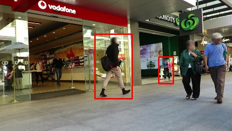
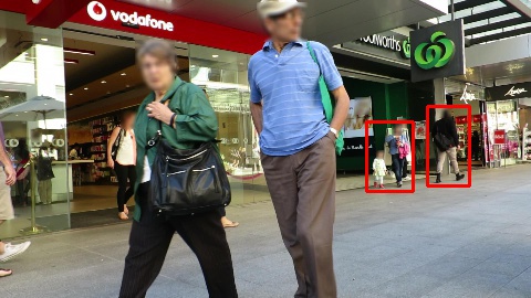
In these frames from the MOT dataset, the man wearing a black top walking away and the woman with the little girl standing at the entrance of the Woolworths shop will disappear behind the couple walking in the direction of the camera in the second and third image. Then as the couple keeps walking towards the camera, they cover the four people walking in front or exiting the vodafone boutique.
Note: This is NOT Numina imagery. Numina sensors are not this close and cannot connect information with this level of identifiability. See our privacy policy for more details.
Detection flaws
Since we’re doing tracking by detection, the performance of the object detector is crucial. Several types of detection errors need to be considered.
False alarms
Even if Deep Learning has greatly improved the performance, state of the art object detectors are still not perfect and regularly misfire, indicating the presence of an object that’s not really there. Falsely detected objects effectively increase the object clutter in the image sequence, making the assignment problem more difficult.
Distractors
Different from a false alarm, distractors are elements of the scene for which there is no good answer to whether they should be part of the foreground or the background. The best example of this are phenomena like the reflection of a pedestrian on a glass, or pictures of persons or cars on an advertisement board.
In this frame from MOT dataset, the red bounding boxes are surrounding real physical persons, whereas the blue bounding boxes correspond either to reflections in the glass or image of a person displayed on a screen. It is very common for a person detector to count these blue-boxed objects as true positives.
Detection gap
It can also happen that the detector fails to detect an object of interest on the scene. These missed detections present a problem, as successful tracking relies on regular updates of each object position. The longer a track stays without update, the higher the uncertainty on the object whereabouts.
Segmentation errors
It can also happen that a bounding box from the detector covers several objects or that a single object is responsible for several detections results.
A common error from an object detector is to undersegment when two objects of the same type are close together. Here, we see two persons in the red bounding box are detected as one.
Sometimes the opposite happens, and an object is oversegmented. The two blue bounding boxes can both be considered true positives as they are explained by the actual presence of a person, but it is one person counted twice. Non-Maximum Suppression usually helps prevent counting the same objects several times, but it does not prevent every occurrence due to inaccuracies in the bounding box estimate.
Appearance descriptors
Finding reliable appearance-matching functions is still an open problem. Due to appearance and illumination changes, a trivial template matching by sum of absolute differences does not work reliably to match objects. Even the use of Normalized Cross Correlation, or features like gradient magnitude, HOG or histograms will regularly generate spurious matches.
Here are two sample images from one of our sensors, separated by a few seconds. Using Normalized-Cross-Correlation, we scan the image on the right, looking for the rectangle that is the most similar to the green rectangle on the left frame. According to that distance metric, it is not the new detection bounding box on the right frame, but the rectangle inside the red box.
Note: Numina only collects high frame rate samples on rare occasions, for Research and Development, and Quality Insurance, and always with explicit, advance authorization from our customer. See our Privacy Policy.
Why does privacy make this harder?
At Numina, as part of our commitment to Intelligence without Surveillance, we process images entirely onboard our sensor hardware and only transmit only anonymized metadata about the tracks. Doing this presents some distinct challenges to our tracking algorithms.
Edge Processing
Real-time edge processing (on remotely deployed hardware, with finite capacity) limits complexity of models both for detection and data association because the available computing power is considerably lower than on a server and our application needs to keep up with the unceasing flow of new images.
In order to accurately represent what is happening in a scene, we need to sample the video feed at a high enough frame rate to account for the normal speed of travel for pedestrians, bicyclists, and vehicles — which limits the amount of computation allowed for each image. On the other hand, we can’t hope to achieve high accuracy without a minimum complexity. Part of our challenge is finding the best tradeoff and designing algorithms that are both efficient and accurate. For this reason, it is important to design purpose-built AI products — in Numina’s case, focused on multimodal object detection and tracking in urban environments.
Privacy First
Our Privacy Policy states that we will never intentionally collect personally identifiable information. We take this commitment seriously, and believe it applies not just to the metadata transmitted, but also to information represented in intermediate stages of processing. When designing an appearance descriptor that allows us to recognize the same object in different images, we try to ensure we aren’t creating any information that could be used to identify a person (for example, facial recognition descriptors, or license plate numbers).
The Why of the Where
At Numina, we’re excited to solve these engineering problems with the end mission of making places more responsive, walkable, bikeable, and equitable. Because Numina deploys in the public realm, it is paramount that we develop this AI responsibly. If you’d like to get involved, let us know at join@numina.co!
References:
- https://numina.co/our-privacy-principles/
- Leal-Taixé, Laura, et al. “Tracking the trackers: an analysis of the state of the art in multiple object tracking.” arXiv preprint arXiv:1704.02781 (2017).
- Milan, Anton, et al. “MOT16: A benchmark for multi-object tracking.” arXiv preprint arXiv:1603.00831 (2016).
- https://motchallenge.net/
- Zhang, Li, Yuan Li, and Ramakant Nevatia. “Global data association for multi-object tracking using network flows.” 2008 IEEE Conference on Computer Vision and Pattern Recognition. IEEE, 2008.
- Kim, Chanho, et al. “Multiple hypothesis tracking revisited.” Proceedings of the IEEE International Conference on Computer Vision. 2015.
